
Distributed tracing is a method to track and analyze the journey of a single request across multiple microservices, making it easier to identify and resolve performance bottlenecks. It assigns unique identifiers to requests, creating a detailed map of interactions between services, APIs, and databases. This approach is vital for diagnosing delays in complex systems, especially in modern microservice architectures where traditional monitoring tools fall short.
Key Highlights:
- How It Works: Distributed tracing uses unique Trace IDs and spans to visualize a request’s path, pinpointing slowdowns in specific services or components.
- Core Components: Traces (complete request journey), spans (individual operations), and trace context (links spans across services).
- Benefits: Reduces debugging time, improves Mean Time to Detection (MTTD) and Mean Time to Resolution (MTTR), and provides clear visibility into system performance.
- Tools and Standards: OpenTelemetry is a popular framework for implementing tracing, replacing older systems like OpenTracing.
- Common Issues Identified: N+1 query patterns, cascading latency, fan-out bottlenecks, and silent timeouts.
The Anatomy of a Distributed Trace
What is Distributed Tracing?
Distributed tracing follows a single request as it moves through multiple services, assigning unique identifiers to each user action. This allows precise tracking to pinpoint where time is spent and identify delays along the way.
At its core, distributed tracing revolves around three elements: traces, spans, and trace context. A trace represents the entire journey of a request from start to finish, often visualized as a waterfall chart that highlights every operation. A span focuses on a specific task, such as an API call, a database query, or a function execution. Each span includes details like the operation name, timestamps, and metadata about what occurred. The trace context ties it all together using unique identifiers – Trace ID and Span ID – which are passed between services, usually through HTTP headers.
Let’s break down these concepts further to understand how distributed tracing works.
Traces, Spans, and Context Explained
Traces, spans, and context work in harmony to map out a request’s journey. Imagine a user clicking "Submit Order." That action gets assigned a Trace ID, like 4bf92f3577b34da6a3ce929d0e0e4736, which stays with the request throughout its lifecycle.
When the request hits your API gateway, a span is created to log the interaction. This span includes its own Span ID, the Trace ID it belongs to, timestamps, and metadata like the HTTP method used. As the API gateway calls the payment service, it passes the Trace ID in a header called traceparent. The payment service picks up this context, creates its own span with a new Span ID, and records the original span’s ID as its "Parent ID." This process repeats across all service interactions – like database queries or external API calls – building a detailed hierarchy of the request.
The W3C Trace Context standard defines how this information is passed along. The traceparent header has a specific format: version-traceId-parentId-traceFlags. For instance: 00-4bf92f3577b34da6a3ce929d0e0e4736-00f067aa0ba902b7-01.
Modern frameworks like OpenTelemetry have largely replaced older systems like OpenTracing and OpenCensus. OpenTelemetry categorizes spans into five types based on their role:
| Span Kind | Type | Common Examples |
|---|---|---|
| Server | Synchronous | HTTP server handlers, gRPC server calls |
| Client | Synchronous | Outgoing HTTP requests, database queries |
| Producer | Asynchronous | Publishing to Kafka, RabbitMQ, or SQS |
| Consumer | Asynchronous | Processing messages from queues or topics |
| Internal | In-process | Business logic, data transformations |
Understanding these span types helps pinpoint which operations contribute to latency.
Another powerful feature is baggage – custom key-value pairs like customer_id or session_id that travel with the trace across services. This extra data allows for more refined filtering and faster problem identification.
Grasping these components is essential to see how distributed tracing simplifies troubleshooting.
Why Distributed Tracing Matters
As microservices become the norm, distributed tracing has gone from optional to essential. Back in 2020, 61% of enterprises had adopted microservices. By 2023, 84% were using or exploring Kubernetes. In these systems, a single user action can trigger dozens of backend operations across various teams and servers.
Traditional monitoring tools fall short here. Metrics can tell you what’s happening – like a sudden spike in response times – while logs explain why something failed, such as a database timeout. But traces go a step further, showing exactly where the issue lies in the request chain.
"Distributed tracing eliminates individual service’s data silos and reveals what’s happening outside of service borders." – Elastic
This visibility drastically reduces debugging time. Instead of spending hours piecing together logs from different services, you get a clear waterfall view of events. For instance, you might find that a 12-second checkout delay stems from a 9-second database query in the inventory service.
High-throughput systems generate millions of spans per minute, which is why many teams use tail-based sampling. This method retains traces with errors or high latency while sampling normal requests. To keep observability systems efficient, it’s recommended to limit unique span names to under 1,000.
Distributed tracing also provides service dependency mapping. By analyzing how services interact and how frequently, tracing tools can automatically generate visual diagrams of your system’s architecture. These diagrams help identify critical paths and understand how delays in one service can ripple through the entire request flow.
Setting Up Distributed Tracing
To set up distributed tracing, start by initializing a TracerProvider, configuring exporters, adding span processors, and acquiring a tracer. Once that’s done, you can begin creating spans to monitor and track operations effectively.
OpenTelemetry offers two approaches to instrumentation: automatic and manual. Automatic instrumentation uses prebuilt agents or extensions to integrate with common frameworks like PHP, Node.js, Java, and Python. On the other hand, manual instrumentation allows you to define custom spans for more specialized use cases.
Automatic vs. Manual Instrumentation
Automatic instrumentation is the quickest way to get started. With agents or extensions, it captures common operations such as HTTP requests or database queries without requiring code changes.
However, manual instrumentation comes into play when you need to track unique operations or use unsupported frameworks. Here’s how it works in different languages:
- Python: Use
tracer.start_as_current_span("operation_name")as a context manager to handle the span lifecycle automatically. - Node.js: Create spans with
tracer.startSpan("name", { kind: trace.SpanKind.SERVER })and manage context usingcontext.with()to ensure child spans are linked correctly. - Go: Pass context explicitly as a function argument since implicit propagation isn’t supported.
| Feature | Automatic Instrumentation | Manual Instrumentation |
|---|---|---|
| Effort | Low; often just involves installing an agent | High; requires code changes and API usage |
| Coverage | Broad; supports common frameworks and libraries | Specific; tailored to custom business logic |
| Control | Limited to agent capabilities | Detailed; allows custom attributes and spans |
| Use Case | Standard HTTP/DB operations | Custom protocols or complex workflows |
Once you’ve chosen your instrumentation method, fine-tune your setup for optimal performance and consistency.
Configuration Best Practices
When naming spans, keep them short and generic to avoid performance issues. Ideally, limit the number of unique span names to fewer than 1,000. Follow OpenTelemetry’s semantic conventions for attributes, using standardized names like http.method, db.system, and net.peer.ip for consistency across services.
For systems with heavy traffic, consider head-based sampling to manage data volume. For example, a 5% sampling rate records one out of every 20 traces, which helps reduce costs while still providing enough data for analysis. In production, use a BatchSpanProcessor to send spans in batches, improving efficiency compared to sending them individually. Assign the correct SpanKind (Server, Client, Producer, Consumer, or Internal) to help tracing backends map service dependencies accurately.
Finally, ensure proper trace context propagation. Adhering to the W3C Trace Context standard ensures that Trace IDs and Span IDs are maintained across service boundaries. For asynchronous operations, explicitly pass context to preserve trace connections and avoid breaking the trace chain.
Finding Latency Issues with Traces
Distributed tracing can be a game-changer when it comes to identifying performance slowdowns. By combining precise querying techniques with visualization tools, you can uncover bottlenecks that might be hidden within aggregated metrics. Here’s a closer look at how to focus on slow requests and connect traces with logs and metrics to diagnose issues effectively.
Querying and Filtering Slow Requests
Start by zeroing in on traces that exceed specific duration thresholds. For example, if your system’s typical response time is under 500 ms, filter for traces taking longer than 1 second to identify outliers. You can also correlate latency with outcomes by filtering traces based on status codes. For instance, if high latency consistently aligns with 5xx errors, it’s a strong indicator that delays are tied to failures rather than standard processing.
Use attribute filters like service.name, http.status_code, and host.id to determine whether the issue is tied to a specific microservice or infrastructure component. In high-traffic environments, latency heatmaps can make rare but severe outliers easier to spot. Once you’ve identified a slow request, locate its unique Trace ID to pull up an end-to-end visualization in your trace explorer. Tail-based sampling, which analyzes traces after completion, is often preferred over head-based sampling for its ability to capture complete data sets.
Connecting Traces with Logs and Metrics
Traces reveal where delays occur, but logs often explain why. This connection hinges on trace ID injection – embedding unique identifiers like trace_id and span_id into your application logs. This allows you to filter and review logs for specific slow requests. Many modern observability platforms use the W3C Trace Context standard and the traceparent header to propagate trace identifiers across service boundaries. Pairing this with unified service tagging (using tags like env, service, and version) makes it easier to link latency spikes in metrics to the exact traces and logs from that time.
Structured logging in JSON format ensures trace data can be indexed and queried efficiently. When you notice a latency spike, use timestamps and tags to isolate relevant traces and logs. You can also link traces to infrastructure metrics by including attributes like host or container IDs. This approach helps determine whether slowness is due to application code issues or resource constraints, such as high CPU usage.
"Tracing context that comes into a service with a request is propagated to other processes and attached to transaction data. With this context, you can stitch the transactions together later."
- Erika Arnold, Software Architect
Combining these methods with visual tools provides even deeper clarity into performance issues.
Reading Trace Visualizations
Trace visualizations like waterfall charts break down the end-to-end journey of a request into individual spans, each with distinct start and end timestamps. These horizontal bars show how time is distributed across services or database queries, making bottlenecks easy to spot. For example, if a database span takes 800 ms within a 1-second request, that’s likely a key issue.
Service dependency maps provide a clear overview of how services interact, showing upstream and downstream dependencies. These maps can highlight which service in the chain is causing delays, offering a visual "map" of microservice calls. Similarly, flame graphs display the call hierarchy, with longer bars indicating areas where more time is being spent.
During active incidents, consider enabling 100% sampling temporarily to ensure no critical data is missed. Adding business-relevant metadata – like user_id, order_id, or environment – to spans allows for more targeted analysis. This can help you determine whether performance issues are widespread or limited to specific user groups or scenarios.
sbb-itb-0fa91e4
Root Cause Analysis Techniques
After identifying a slow trace, the next step is figuring out what’s causing the issue. By combining trace visuals and context propagation methods with manual analysis and modern debugging tools, you can quickly pinpoint and address the root of latency problems.
Examining Span Durations and Service Dependencies
Start by focusing on the critical path – the spans that take up the most time in the overall request. Waterfall charts are particularly useful here, as they show exactly how much time each operation contributes to the total latency.
Different span types can help you zero in on the source of delays:
- Server spans handle incoming requests.
- Client spans represent outbound calls, like database queries or API requests.
- Internal spans track in-process tasks like business logic.
By comparing a Client span to its corresponding Server span, you can figure out if the delay is due to internal processing or network overhead.
Keep an eye out for common patterns in your traces. For example:
- N+1 query patterns: Repeated database queries running in sequence often point to inefficient ORM usage.
- Silent timeouts: A single long-duration span with no child activity may indicate overly generous timeout settings.
- Cascading latency: Sequential spans with growing delays could signal resource contention downstream.
- Fan-out bottlenecks: When one slow parallel call determines the overall response time.
Service dependency maps are also key. They show how services interact and help uncover redundant hops. Filtering spans by attributes like user ID, database statement, or HTTP route can reveal whether the issue affects all users or just specific segments. These insights make it easier to focus your efforts.
Applying the 5 Whys Method
The 5 Whys technique pairs perfectly with distributed tracing. By repeatedly asking "why", you can drill down to the root cause of an issue. Here’s an example:
- Why is checkout slow? The trace shows the Payment Service is slow.
- Why is the Payment Service slow? A child span points to a 134 ms database query.
- Why is the database query slow? The span’s attributes highlight a specific SQL statement.
- Why is that SQL statement slow? Logs reveal lock contention.
This method transforms vague complaints into specific, actionable problems. Each "why" takes you deeper into the trace, from high-level service delays to specific database queries or API calls. Adding metadata like customer ID, host, or SQL statements gives even more clarity.
"Distributed tracing is the connective tissue between metrics and logs. Without it, you’re working with disconnected data points."
- Faiz Shaikh
This structured approach not only simplifies debugging but also lays the groundwork for automated insights using tools like TraceKit.
Using TraceKit for Faster Debugging
While manual analysis is valuable, modern tools like TraceKit can speed things up. TraceKit uses flame graphs and AI-driven anomaly detection to surface performance issues automatically, saving you from manually inspecting every span. It highlights key attribute correlations, making it easier to find the root cause.
One standout feature of TraceKit is live breakpoints. These allow you to capture variable states in production code without needing to redeploy. This is especially helpful when a trace points to a bottleneck but doesn’t explain the underlying issue – like a memory overflow or a blocking operation. By setting a live breakpoint on the slow span, you can capture real-time variable values and diagnose the problem without adding extra logging or restarting services.
TraceKit also provides service dependency maps and request waterfall visualizations, making it simple to spot fan-out problems, circular dependencies, or missing instrumentation. With support for languages like PHP, Node.js, Go, Python, Java, and Ruby, TraceKit can automatically instrument popular frameworks like Laravel and Express, minimizing setup time. This automation is especially useful for high-throughput systems generating millions of spans per minute.
Step-by-Step Latency Troubleshooting
Step-by-Step Distributed Tracing Latency Troubleshooting Process
Using the tracing techniques and practices discussed earlier, here’s how to systematically diagnose and resolve latency issues.
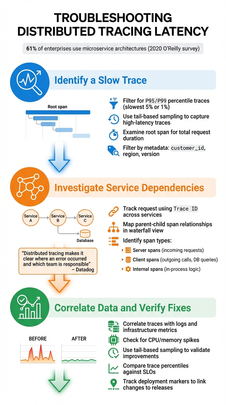
Step 1: Identify a Slow Trace
Start by narrowing your focus to the slowest traces. Use your monitoring tools to filter for traces in the P95 or P99 percentiles – these represent the slowest 5% or 1% of requests that are likely impacting user experience. Tail-based sampling is particularly helpful here, as it ensures you capture all high-latency or error-prone traces.
Look at the root span, which represents the entire request duration. This span shows the total time taken from the start of the first operation to the completion of the last one. Tools like flame graphs and waterfall visualizations can make this process easier. The root span appears at the top, with nested child spans below, clearly showing how long each service or database call took.
You can also filter traces by metadata, such as customer_id, region, or version, to see if the latency affects all users or specific groups. If you’re struggling to find slow traces, check your sampling strategy. Probabilistic sampling (e.g., capturing 1 in 1,000 traces) might miss the exact requests you need to investigate.
Once you’ve identified a slow trace, follow its path through the system to locate the bottleneck.
Step 2: Investigate Service Dependencies
Using the slow trace as your starting point, map out the request’s journey to locate where delays are occurring. Use the Trace ID to track the request as it moves across services. In waterfall visualizations, you’ll see a parent-child relationship between spans: a client span in one service corresponds to a server span in the next. This structure helps you pinpoint where delays originate.
Pay close attention to span types:
- Server spans: Handle incoming requests.
- Client spans: Represent outgoing synchronous calls, such as database queries or API requests.
- Internal spans: Track in-process logic within a single service.
"Distributed tracing makes it clear where an error occurred and which team is responsible for fixing it." – Datadog
By identifying the specific service or operation causing the delay, you can focus your troubleshooting efforts on the right area.
Step 3: Correlate Data and Verify Fixes
Once you’ve isolated the problematic span, correlate it with logs and metrics to confirm your findings. For example, compare traces with infrastructure metrics to identify resource constraints, such as CPU or memory spikes.
After implementing a fix, use tail-based sampling to validate improvements. Keep an eye on trace percentiles and compare them against your service level objectives (SLOs) to ensure performance stays within acceptable limits. You can also track deployment markers in your tracing system to directly link performance changes to specific code releases.
A 2020 O’Reilly survey found that 61% of enterprises use microservice architectures, which makes having a structured approach to managing service interactions even more critical. By consistently following these steps, you can turn vague performance issues into clear, data-driven solutions.
Conclusion
Distributed tracing provides a clear, end-to-end view of how requests travel through your system, eliminating the need to guess where latency originates or dig through disconnected logs. Instead of reacting to problems as they arise, this method allows you to anticipate and address bottlenecks before they escalate into alerts or impact user experiences.
This guide has walked through practical techniques for effective tracing and analysis. From grasping spans and context propagation to using the 5 Whys method and correlating telemetry, these steps create a structured framework for pinpointing root causes. When paired with smart sampling and standardized instrumentation, these strategies not only lower Mean Time to Detect (MTTD) and Mean Time to Resolve (MTTR) but also help manage costs efficiently.
"Distributed tracing is no longer a ‘nice-to-have’ feature; it’s an essential survival tool for modern engineering teams." – Nitya Timalsina, Developer Advocate, OpenObserve
FAQs
How does distributed tracing help identify and resolve issues in microservices?
Distributed tracing offers a complete view of how a request travels through your microservices. By dividing each request into timed spans, it reveals exactly where delays or errors occur, helping developers zero in on the root cause without depending entirely on logs or general monitoring tools.
This method cuts down debugging time by identifying problem areas like sluggish services or failing operations. It also provides a clear picture of service dependencies and performance issues, making it a vital resource for keeping complex distributed systems running smoothly.
What’s the difference between automatic and manual instrumentation in distributed tracing?
When it comes to integrating tracing into your system, you have two main approaches: automatic instrumentation and manual instrumentation.
Automatic instrumentation uses built-in agents tailored for popular frameworks, making it easy to implement with minimal code changes. It’s a fast and straightforward way to get started, especially for standard use cases where basic tracing is sufficient.
Manual instrumentation, however, gives developers the ability to add custom tracing code. This approach provides more control and allows for capturing highly specific or detailed data. While it offers flexibility, it does require more effort and time to implement.
Often, a combination of both methods works best. Automatic instrumentation can handle routine tasks, while manual instrumentation can be used for more complex systems or when deeper insights are needed. It all depends on the complexity of your setup and your debugging needs.
How does distributed tracing help pinpoint performance issues in a system?
Distributed tracing works like a detailed map, tracking every request as it moves through a system. It assigns each transaction a unique trace ID and breaks it down into spans – timed segments representing specific operations such as API calls, database queries, or cache lookups. By visualizing these spans, engineers can pinpoint the source of latency, whether it’s tied to a particular service, API endpoint, or database query.
When paired with system metrics like CPU usage, memory consumption, or network activity, distributed tracing becomes even more powerful. For instance, a span that’s consistently slow might align with high CPU usage or indicate a database bottleneck, making it easier to locate the exact issue. Tools like TraceKit take this further by capturing live variable states and presenting performance data through flame graphs. This helps teams quickly identify and resolve bottlenecks without needing to redeploy code, transforming vague performance issues into clear, actionable fixes.